Time Averaging of 1-min Data (floor / ceiling / center)#
This notebook loads one monthly archive (§2), runs the same solpos → clear-sky → ``qc_test`` → ``qc_mask`` pipeline as ``2.quality_control.ipynb`` in brief (§3), then shows averaging on the dataset via ``BSRNDataset.average`` (§4). The rest focuses on ``pretty_average`` and direct DataFrame use.
§5 explains how pretty_average differs from pandas.resample (windows, monthly label trim, coverage, match_ceiling_labels); §5.1 uses ``ds.data()`` (QC-masked minute data after §3) for alignments; §5.2 compares ``match_ceiling_labels`` for center only; §5.3 tabulates samples per 1 h interval (floor / ceiling / center). §6 applies 1 h averaging to the QIQ month. §7–8 plot comparisons (plots at the end of the workflow).
1. Import libraries#
[ ]:
import os

import matplotlib.pyplot as plt
import pandas as pd

import bsrn
from bsrn.utils import pretty_average

INPUT_FILE = "/Volumes/Macintosh Research/Data/bsrn-qc/data/QIQ/qiq0824.dat.gz"

pd.options.display.max_columns = None
2. Load QIQ August data#
[2]:
if os.path.exists(INPUT_FILE):
    ds = bsrn.BSRNDataset.from_file(INPUT_FILE)
    stn = ds.station_code
    print(
        f"Data for {stn} loaded successfully ({ds.year}-{ds.month:02d})."
    )
    display(ds.data().head())
else:
    raise FileNotFoundError(
        f"File not found: {INPUT_FILE}. Current working directory: {os.getcwd()}"
    )
Data for QIQ loaded successfully (2024-08).
| ghi | bni | dhi | lwd | temp | rh | pressure | |
|---|---|---|---|---|---|---|---|
| 2024-08-01 00:00:00+00:00 | 105.0 | 0.0 | 106.0 | 421.0 | 25.2 | 70.0 | 981.0 |
| 2024-08-01 00:01:00+00:00 | 108.0 | 0.0 | 109.0 | 422.0 | 25.2 | 71.0 | 981.0 |
| 2024-08-01 00:02:00+00:00 | 112.0 | 0.0 | 113.0 | 421.0 | 25.2 | 70.0 | 981.0 |
| 2024-08-01 00:03:00+00:00 | 113.0 | 0.0 | 114.0 | 421.0 | 25.2 | 70.0 | 981.0 |
| 2024-08-01 00:04:00+00:00 | 116.0 | 0.0 | 117.0 | 421.0 | 25.2 | 71.0 | 981.0 |
3. Solar geometry, clear-sky (REST2), and QC#
We use the same pipeline as ``2.quality_control.ipynb``: BSRNDataset.solpos, BSRNDataset.clear_sky (here model='rest2' with MERRA-2 via Hugging Face), then BSRNDataset.qc_test followed immediately by BSRNDataset.qc_mask (failed irradiance → NaN, standard flag* columns dropped). Read ``2.quality_control`` for details; we do not tabulate flags here. ``ds.data()`` after §3 is the QC-masked minute frame for ``pretty_average`` from §5 onward;
§4 calls ``average`` on ``ds.model_copy(deep=True)`` so ``ds`` stays at minute resolution.
[3]:
# Same pipeline as 2.quality_control.ipynb
ds.solpos()
ds.clear_sky(model="rest2")
ds.qc_test()
ds.qc_mask()

display(ds.data()[["ghi", "ghi_clear", "zenith"]].head())
Fetching MERRA-2 from Hugging Face: qiq/qiq0824_merra2.parquet
| ghi | ghi_clear | zenith | |
|---|---|---|---|
| 2024-08-01 00:00:00+00:00 | 105.0 | 507.439814 | 54.881 |
| 2024-08-01 00:01:00+00:00 | 108.0 | 509.994881 | 54.717 |
| 2024-08-01 00:02:00+00:00 | 112.0 | 512.545982 | 54.553 |
| 2024-08-01 00:03:00+00:00 | 113.0 | 515.077560 | 54.390 |
| 2024-08-01 00:04:00+00:00 | 116.0 | 517.620641 | 54.226 |
4. Pipeline averaging: BSRNDataset.average#
On a ``BSRNDataset``, call ``average(freq, …)`` on the dataset (not on the bare DataFrame from ``data()``). It delegates to ``pretty_average`` on the cached frame, then replaces that cache with the coarser-index result. §5+ still need minute-level ``ds``, so we ``model_copy(deep=True)`` (Pydantic) and call ``average`` on the copy—same columns as ``ds.data()`` after §3 (including QC-masked irradiance).
When you are done with minute data, you may call ``average`` on ``ds`` itself instead of a copy.
[4]:
from IPython.display import display

ds_h = ds.model_copy(deep=True)
ds_h.average("1h", alignment="ceiling")
display(ds_h.data()[["ghi", "ghi_clear", "zenith"]].head())
| ghi | ghi_clear | zenith | |
|---|---|---|---|
| 2024-08-01 01:00:00+00:00 | 203.385965 | 581.242271 | 49.990333 |
| 2024-08-01 02:00:00+00:00 | 380.630435 | 706.014627 | 41.060483 |
| 2024-08-01 03:00:00+00:00 | 303.216667 | 791.170072 | 33.993883 |
| 2024-08-01 04:00:00+00:00 | 230.416667 | 826.488629 | 30.319967 |
| 2024-08-01 05:00:00+00:00 | 237.150000 | 817.447416 | 31.301850 |
5. What pretty_average does#
bsrn.utils.averaging.pretty_average implements explicit labeled windows — it is NOT pandas.DataFrame.resample. For each output label time L (bin length Δ from freq), data rows are selected with a rule that depends on ``alignment``.
Windows#
Alignment |
Interval |
Role of |
|---|---|---|
floor |
\([L, L+\Delta)\) |
Label at left edge |
ceiling |
\((L-\Delta, L]\) |
Label at right edge |
center |
\([L-\Delta/2+\mathrm{res},\, L+\Delta/2]\) |
Label at center; |
Monthly label trim#
The regular grid from floor(min) … ceil(max) at freq is trimmed so edge bins do not straddle month boundaries (lo / hi from the data index). floor drops labels at the high edge; ceiling drops at the low edge. For center, choose the same trim as ceiling or floor via ``match_ceiling_labels`` (default True).
Coverage#
A numeric aggregate is emitted only if enough rows are “valid” (numeric columns: at least one finite value in that row).
floor / ceiling: valid count must be > half of the nominal step count \(\approx \Delta/\mathrm{res}\).
center: valid count must be > half of rows in the window (not the nominal count).
Otherwise the row is still emitted but values are NaN.
Inputs#
``DatetimeIndex`` is required.
Below: §5.1 uses ``ds.data()`` for floor/ceiling/center; §5.2 compares ``match_ceiling_labels`` (center only); §5.3 counts samples per 1 h window. §6 applies pretty_average for the workflow plots.
5.1 Case A — full month, different label times#
All rows in ``ds.data()`` after §3 (one station-month from the archive). freq='1h': floor / ceiling / center differ in where the hour label sits; counts can differ slightly at month edges.
[5]:
# ds.data() after §3: one station-month (see INPUT_FILE)
df_a = ds.data()[["ghi", "zenith"]].copy()
freq = "1h"

f_a = pretty_average(df_a, freq, alignment="floor")
c_a = pretty_average(df_a, freq, alignment="ceiling")
z_a = pretty_average(df_a, freq, alignment="center")

print("Case A — 1 h labels (UTC) on the loaded month:")
print(f"  native rows in window: {len(df_a)}")
for name, s in [("floor", f_a), ("ceiling", c_a), ("center", z_a)]:
    print(f"  {name:7s}: n={len(s):4d}  first={s.index[0]}  last={s.index[-1]}")
Case A — 1 h labels (UTC) on the loaded month:
  native rows in window: 44640
  floor  : n= 744  first=2024-08-01 00:00:00+00:00  last=2024-08-31 23:00:00+00:00
  ceiling: n= 744  first=2024-08-01 01:00:00+00:00  last=2024-09-01 00:00:00+00:00
  center : n= 744  first=2024-08-01 01:00:00+00:00  last=2024-09-01 00:00:00+00:00
5.2 Case B — match_ceiling_labels usage#
For ``alignment=’center’`` only: ``match_ceiling_labels`` chooses whether monthly label trimming follows ceiling (default) or floor. Compare the two ``center`` outputs (row counts and first/last labels).
[6]:
freq = "1h"
# Same input columns as §5.1; Case B only compares center + match_ceiling_labels
df_b = ds.data()[["ghi", "zenith"]].copy()

z_hi = pretty_average(df_b, freq, alignment="center", match_ceiling_labels=True)
z_lo = pretty_average(df_b, freq, alignment="center", match_ceiling_labels=False)

print("Case B — center only: match_ceiling_labels True vs False")
print(f"  n_row: {len(z_hi)} vs {len(z_lo)}")
print("  first label:", z_hi.index[0], "vs", z_lo.index[0])
print("  last  label:", z_hi.index[-1], "vs", z_lo.index[-1])
Case B — center only: match_ceiling_labels True vs False
  n_row: 744 vs 744
  first label: 2024-08-01 01:00:00+00:00 vs 2024-08-01 00:00:00+00:00
  last  label: 2024-09-01 00:00:00+00:00 vs 2024-08-31 23:00:00+00:00
5.3 Case C — samples per 1 h interval#
For ``freq=’1h’``, each output row is the mean over a time window; the table counts how many native rows fall in that window (``n_samples``) for floor, ceiling, and center (same logic as pretty_average). Labels and counts differ across alignments. Preview tables use ``display()`` so every row renders in the notebook (plain ``print`` on wide tables can be truncated).
[7]:
import bsrn.utils.averaging as av
from IPython.display import display

def hourly_sample_counts(df, freq, alignment, match_ceiling_labels=True):
    """Native rows per 1 h label (same windows as pretty_average)."""
    delta = av._period_delta(freq)
    res = av._archive_timestep_1_or_3(df.index)
    labels = av._label_grid(df.index, freq)
    labels = av._trim_labels_for_alignment(
        labels, df.index, freq, alignment, match_ceiling_labels=match_ceiling_labels,
    )
    idx = df.index
    rows = []
    for L in labels:
        m = av._window_mask(idx, L, delta, alignment, res)
        rows.append((L, int(m.sum())))
    return pd.DataFrame(rows, columns=["label_utc", "n_samples"])


freq = "1h"
dfc = ds.data()[["ghi", "zenith"]].copy()

floor_ct = hourly_sample_counts(dfc, freq, "floor")
ceil_ct = hourly_sample_counts(dfc, freq, "ceiling")
cent_ct = hourly_sample_counts(dfc, freq, "center", match_ceiling_labels=True)

print("Case C — n_samples per 1 h interval (native rows in each window)")
# display() renders full HTML tables (avoids stdout truncation in long cells).
# display() renders full HTML tables (avoids stdout truncation in long cells).
print("\nfloor — head 4:")
display(floor_ct.head(4))
print("floor — tail 4:")
display(floor_ct.tail(4))
print("\nceiling — head 4:")
display(ceil_ct.head(4))
print("ceiling — tail 4:")
display(ceil_ct.tail(4))
print("\ncenter (match_ceiling_labels=True) — head 4:")
display(cent_ct.head(4))
print("center — tail 4:")
display(cent_ct.tail(4))

print("\nSummary n_samples (all intervals):")
for name, tab in [("floor", floor_ct), ("ceiling", ceil_ct), ("center", cent_ct)]:
    s = tab["n_samples"]
    print(f"  {name:7s}: count={len(s)}, min={s.min()}, max={s.max()}, mean={s.mean():.1f}")
Case C — n_samples per 1 h interval (native rows in each window)

floor — head 4:
| label_utc | n_samples | |
|---|---|---|
| 0 | 2024-08-01 00:00:00+00:00 | 60 |
| 1 | 2024-08-01 01:00:00+00:00 | 60 |
| 2 | 2024-08-01 02:00:00+00:00 | 60 |
| 3 | 2024-08-01 03:00:00+00:00 | 60 |
floor — tail 4:
| label_utc | n_samples | |
|---|---|---|
| 740 | 2024-08-31 20:00:00+00:00 | 60 |
| 741 | 2024-08-31 21:00:00+00:00 | 60 |
| 742 | 2024-08-31 22:00:00+00:00 | 60 |
| 743 | 2024-08-31 23:00:00+00:00 | 60 |
ceiling — head 4:
| label_utc | n_samples | |
|---|---|---|
| 0 | 2024-08-01 01:00:00+00:00 | 60 |
| 1 | 2024-08-01 02:00:00+00:00 | 60 |
| 2 | 2024-08-01 03:00:00+00:00 | 60 |
| 3 | 2024-08-01 04:00:00+00:00 | 60 |
ceiling — tail 4:
| label_utc | n_samples | |
|---|---|---|
| 740 | 2024-08-31 21:00:00+00:00 | 60 |
| 741 | 2024-08-31 22:00:00+00:00 | 60 |
| 742 | 2024-08-31 23:00:00+00:00 | 60 |
| 743 | 2024-09-01 00:00:00+00:00 | 59 |
center (match_ceiling_labels=True) — head 4:
| label_utc | n_samples | |
|---|---|---|
| 0 | 2024-08-01 01:00:00+00:00 | 60 |
| 1 | 2024-08-01 02:00:00+00:00 | 60 |
| 2 | 2024-08-01 03:00:00+00:00 | 60 |
| 3 | 2024-08-01 04:00:00+00:00 | 60 |
center — tail 4:
| label_utc | n_samples | |
|---|---|---|
| 740 | 2024-08-31 21:00:00+00:00 | 60 |
| 741 | 2024-08-31 22:00:00+00:00 | 60 |
| 742 | 2024-08-31 23:00:00+00:00 | 60 |
| 743 | 2024-09-01 00:00:00+00:00 | 29 |
Summary n_samples (all intervals):
  floor  : count=744, min=60, max=60, mean=60.0
  ceiling: count=744, min=59, max=60, mean=60.0
  center : count=744, min=29, max=60, mean=60.0
6. Apply to QIQ (1 h)#
Same freq and three alignments on the QC-masked August frame (§3). Row counts often differ slightly between alignments.
[8]:
FREQ = "1h"

# Irradiance + zenith (required by pretty_average)
cols_avg = [c for c in ("ghi", "ghi_clear", "zenith") if c in ds.data().columns]
df_in = ds.data()[cols_avg].copy()

avg_floor = pretty_average(df_in, FREQ, alignment="floor")
avg_ceil = pretty_average(df_in, FREQ, alignment="ceiling")
avg_center = pretty_average(df_in, FREQ, alignment="center")

print("Row counts — floor:", len(avg_floor), "ceiling:", len(avg_ceil), "center:", len(avg_center))
Row counts — floor: 744 ceiling: 744 center: 744
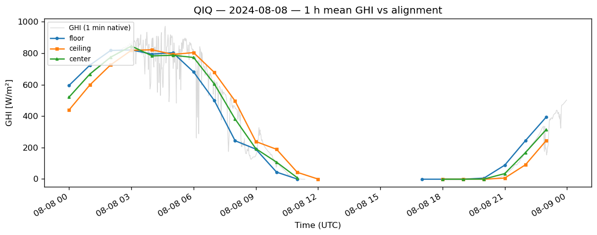
7. Plots: compare GHI means#
Run §6 first so avg_floor, avg_ceil, and avg_center exist.
Overlay 1-hour mean GHI for the three alignments on a short slice (2024-08-08 UTC).
[9]:
day = "2024-08-08"
sub = slice(f"{day} 00:00", f"{day} 23:59")

fig, ax = plt.subplots(figsize=(10, 4), dpi=120)

if "ghi" in ds.data().columns:
    ax.plot(
        ds.data().loc[sub].index,
        ds.data().loc[sub, "ghi"],
        color="0.85",
        linewidth=0.8,
        label="GHI (1 min native)",
    )

ax.plot(avg_floor.loc[sub].index, avg_floor.loc[sub, "ghi"], marker="o", markersize=3, label="floor")
ax.plot(avg_ceil.loc[sub].index, avg_ceil.loc[sub, "ghi"], marker="s", markersize=3, label="ceiling")
ax.plot(avg_center.loc[sub].index, avg_center.loc[sub, "ghi"], marker="^", markersize=3, label="center")

ax.set_ylabel("GHI [W/m²]")
ax.set_xlabel("Time (UTC)")
ax.set_title(f"{stn} — {day} — 1 h mean GHI vs alignment")
ax.legend(loc="upper left", fontsize=8)
fig.autofmt_xdate()
plt.tight_layout()
plt.show()
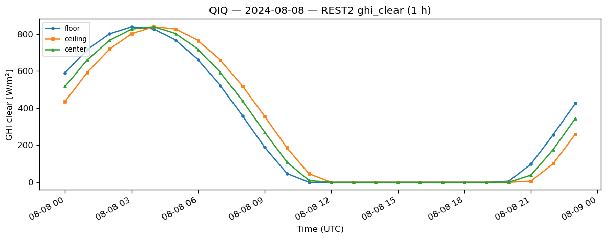
8. Optional: compare clear-sky GHI#
Same overlay for ``ghi_clear`` (REST2).
[10]:
if "ghi_clear" in avg_floor.columns:
    fig, ax = plt.subplots(figsize=(10, 4), dpi=120)
    ax.plot(avg_floor.loc[sub].index, avg_floor.loc[sub, "ghi_clear"], marker="o", markersize=3, label="floor")
    ax.plot(avg_ceil.loc[sub].index, avg_ceil.loc[sub, "ghi_clear"], marker="s", markersize=3, label="ceiling")
    ax.plot(avg_center.loc[sub].index, avg_center.loc[sub, "ghi_clear"], marker="^", markersize=3, label="center")
    ax.set_ylabel("GHI clear [W/m²]")
    ax.set_xlabel("Time (UTC)")
    ax.set_title(f"{stn} — {day} — REST2 ghi_clear (1 h)")
    ax.legend(loc="upper left", fontsize=8)
    fig.autofmt_xdate()
    plt.tight_layout()
    plt.show()